Mastering Looker Studio: A Comprehensive Guide to Calculated Fields

Looker Studio (formerly Google Data Studio) empowers users to transform raw data into insightful reports and dashboards. A key feature in this transformation is the calculated field. Calculated fields allow you to create new dimensions and metrics derived from your existing data, enabling deeper analysis and more tailored visualizations. This guide will walk you through understanding, creating, and managing calculated fields in Looker Studio, complete with illustrative examples and best practices.

Understanding Calculated Fields in Looker Studio

At its core, a calculated field is a formula that performs an action on one or more existing fields in your data source. These actions can range from simple arithmetic operations (like addition or subtraction) and data manipulation with functions (like extracting a date part or concatenating text strings) to implementing branching logic using CASE statements.

Calculated fields are invaluable when the data you need for your reports isn’t directly available in your raw dataset. They allow you to:

• Derive new metrics: Calculate key performance indicators (KPIs) like conversion rates, profit margins, or average order value.
• Transform existing dimensions: Clean up data, reformat text, extract specific information (e.g., a campaign name from a URL), or group values.
• Implement custom logic: Categorize data based on specific conditions or create custom groupings.

By leveraging calculated fields, you can significantly enhance the flexibility and analytical power of your Looker Studio reports, turning standard datasets into actionable insights.

Types of Looker Studio Calculated Fields

Looker Studio offers two primary types of calculated fields, distinguished by where they are created and how they can be used:

1. Data Source Calculated Fields: These fields are created directly within the data source itself.
   • Scope: Once created, they become a permanent part of that data source’s schema and are available for use in any report that connects to that data source.
   • Reusability: Highly reusable across multiple reports and charts.
   • Permissions: Require edit access to the data source to create or modify.
   • Limitations: Generally cannot be used with blended data sources directly within the data source calculation.
2. Chart-Level (or Report-Level) Calculated Fields: These fields are created directly within a specific chart or control in a Looker Studio report.
   • Scope: They exist only within the specific chart or report element in which they were created. They are not added to the underlying data source schema.
   • Reusability: Limited to the specific chart or copied versions of that chart.
   • Permissions: Can be created by report editors, even if they don’t have edit access to the data source.
   • Flexibility: Can be used with blended data sources and are useful for report-specific calculations.
   • Limitation: Cannot be directly referenced by other chart-level calculated fields within the same chart.

Essentially, if a new metric or dimension will be broadly useful across many reports using the same data, creating it as a data source calculated field is more efficient. If the calculation is specific to a particular visualization or involves blended data, a chart-level calculated field is the appropriate choice.

Differentiating Between Data Source and Chart-Level Calculated Fields

The decision of whether to create a data source calculated field or a chart-level one depends on your specific needs and how you intend to use the new field. Here’s a table summarizing the key differences:

Feature	Data Source Calculated Field	Chart-Level Calculated Field
Creation Location	Within the data source	Within a specific chart/control in a report
Availability	In any report using that data source	Only in the specific chart it was created in
Reusability	High (across reports and charts)	Low (specific to the chart)
Permissions Required	Edit rights to the data source	Edit rights to the report
Impact on Data Source	Adds the field to the data source schema	Does not modify the data source schema
Use with Blended Data	No (cannot be created using blended data)	Yes
Referencing Other Calculated Fields	Can reference other data source calculated fields	Cannot reference other chart-level calculated fields in the same chart
Visibility in Field Panel	Appears as a standard field in the data panel	Often indicated with an ‘fx’ symbol or similar in the chart’s setup panel

When to choose which:

• Choose Data Source Calculated Fields when:
  • The new field represents a fundamental metric or dimension that will be useful across multiple reports or by different users of the data source.
  • You want to maintain consistency in how a particular value is calculated across all reports.
  • You need to reference other calculated fields within its formula.
• Choose Chart-Level Calculated Fields when:
  • The calculation is specific to a single chart or a particular analysis within a report.
  • You are working with blended data sources and need to perform calculations across them.
  • You don’t have edit access to the original data source but need to create a derived field for your report.
  • You need to quickly experiment with different calculations without altering the underlying data source.

Step-by-Step Guide to Creating Calculated Fields: Data Source Level

Creating calculated fields at the data source level makes them reusable across any report utilizing that data.

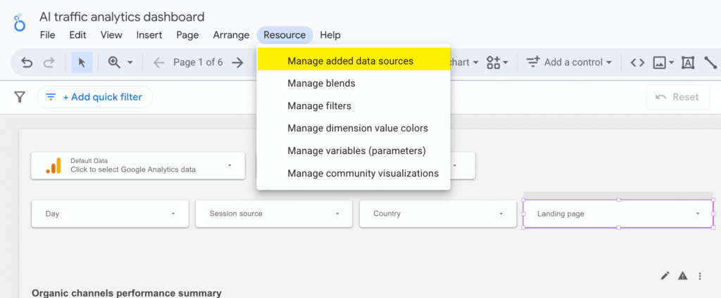
1. Access Your Data Source:

• Open your Looker Studio report.
• In the menu, navigate to “Resource” > “Manage added data sources.”

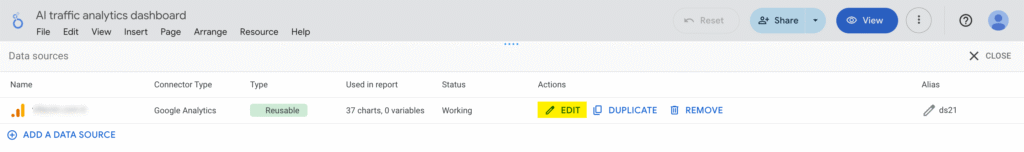
2. Find the data source you want to modify and click “EDIT.” This will open the data source editor.

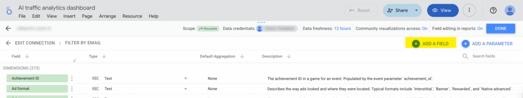
3. Add a New Field:

• In the data source editor, in the upper right corner, click the “+ ADD A FIELD” button.

4. Define the Calculated Field

• A new screen will appear for defining your calculated field.
• Field Name: Enter a descriptive name for your new field (e.g., “Revenue per User,” “Campaign Group”). This name must be unique within the data source.
• Formula: This is where you’ll write the logic for your calculation. You can use:
  • Existing fields from your data source (they will appear in an “Available Fields” list, and you can type to search or drag them into the formula).
  • Mathematical operators (+, -, *, /).
  • Functions (Looker Studio offers a wide range of functions for text, date, aggregation, etc. Start typing a function name, and Looker Studio will provide suggestions).
  • CASE statements for conditional logic.

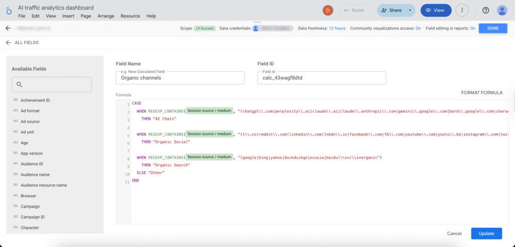
• As you type your formula, Looker Studio will validate the syntax. A green checkmark below the formula box indicates a valid formula. If there are errors, a message will appear.

5. Set Data Type and Aggregation (Crucial!):

• Type: Based on your formula, Looker Studio will often infer the data type (e.g., Number, Text, Boolean, Date). Ensure this is correct. You can change it using the “Type” dropdown if needed (e.g., from Number to Currency or Percent).
• Aggregation: This determines how the field will be summarized if it’s a metric.
  • For formulas that already include an aggregation function (e.g., SUM(Sales), COUNT_DISTINCT(Users)), the default aggregation is usually “Auto,” which is correct. Looker Studio handles the aggregation based on the function used.
  • If your formula operates on unaggregated row-level data (e.g., Price * Quantity, CASE WHEN Category = ‘A’ THEN ‘Group1’ ELSE ‘Group2’ END), the default aggregation might be “Sum” for numeric outputs or “None” or “Count Distinct” for text outputs. Adjust this as needed for how you intend to use the field in charts. For instance, a calculated dimension (like “Campaign Group”) would typically have an aggregation of “None” or be used as a dimension directly. A calculated metric like “Item Revenue” (Price * Quantity) would usually have its default aggregation set to “Sum” to see the total item revenue when used in a scorecard or as a metric in a table.

6. Save the Calculated Field:

• Once you’re satisfied with the name, formula, type, and aggregation, click “SAVE” in the bottom right corner (or “UPDATE” if you are editing an existing field).
• Your new calculated field will now appear in the list of fields for that data source and can be used in any report connected to it. Click “ALL FIELDS” to return to the main data source editor view. Then click “DONE” in the top right to close the data source editor.

Step-by-Step Guide to Creating Calculated Fields: Chart-Level

Chart-level calculated fields are useful for specific visualizations or when working with blended data.

1. Select or Add a Chart:

• Open your Looker Studio report in edit mode.
• Select an existing chart you want to add a calculated field to, or add a new chart to your report canvas.

2. Access the Chart’s Setup Panel:

• With the chart selected, its properties panel will appear on the right side of the screen. Ensure you are in the “SETUP” tab of this panel.

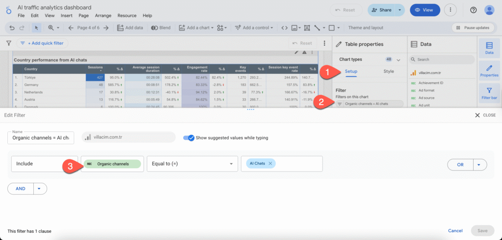
3. Add a New Dimension or Metric:

• Depending on whether you want to create a calculated dimension or a calculated metric, scroll down in the “SETUP” panel to the “Dimension” or “Metric” section.
• Click on “+ Add dimension” or “+ Add metric.”

4. Create a New Field:

• At the bottom of the list of available fields that pops up, click “CREATE FIELD.”

5. Define the Calculated Field:

• A formula editor similar to the data source level will appear.
• Name: Give your chart-level calculated field a descriptive name.
• Formula: Enter your formula using existing fields from the chart’s data source(s), operators, and functions.
  • If using blended data, you can reference fields from any of the blended sources.
  • Important: You cannot reference other chart-level calculated fields within this formula, even if they are defined in the same chart.
• A green checkmark will indicate a valid formula.

5. Set Data Type and Aggregation (if applicable):

• Similar to data source calculated fields, review and adjust the “Type” and “Default Aggregation” as needed. For chart-level fields, the aggregation type you choose here directly impacts how it’s displayed in that specific chart.
• You may also have options for “Display Format” (e.g., for numbers, dates) directly in the chart setup for this field.

6. Apply the Calculated Field:

• Click “APPLY” in the bottom right corner.
• The new calculated field will be added to your selected chart as a dimension or metric. It will only exist and be usable within this specific chart. If you copy this chart, the calculated field will be copied with it.

Editing and Managing Existing Calculated Fields

Over time, you may need to modify or remove calculated fields.

Editing Data Source Calculated Fields:

1. Go to “Resource” > “Manage added data sources.”
2. Click “EDIT” next to the relevant data source.
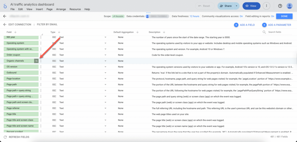
3. In the list of fields, find your calculated field. It will usually have an fx symbol next to its name, indicating it’s a calculated field.
4. Click on the fx symbol (or sometimes directly on the field name if it’s presented as a link) to open the formula editor.
5. Modify the “Field Name,” “Formula,” “Type,” or “Aggregation” as needed.
6. Click “UPDATE” (or “SAVE”) to save your changes.
7. Click “DONE” to close the data source editor. Changes will propagate to all reports using this data source (they might need a refresh).

Editing Chart-Level Calculated Fields:

1. Select the chart that contains the chart-level calculated field.
2. In the chart’s “SETUP” panel, locate the calculated field (either in the Dimension or Metric section). It will typically have an fx symbol next to its name.
3. Click on the fx symbol (or the field name itself). This will open the formula editor for that chart-specific field.
4. Make your modifications to the “Name” or “Formula.”
5. Click “APPLY.” The changes will take effect immediately in that chart.

Managing Calculated Fields (General):

• Deleting Data Source Calculated Fields: In the data source editor, you can typically find a way to delete fields (often an ‘X’ icon or a three-dot menu next to the field). Be cautious, as this will break any reports or charts currently using that field.
• Deleting Chart-Level Calculated Fields: In the chart’s “SETUP” panel, you can usually remove a dimension or metric by clicking an ‘X’ next to it. This removes it from that chart.
• Duplicating: While you can’t directly “duplicate” a data source calculated field in one click to make a variation, you can create a new one and copy-paste the formula as a starting point. For chart-level fields, copying the entire chart will duplicate the field within the new chart.

How Does Aggregation Work in Custom Fields?

Aggregation is the process of summarizing data. In Looker Studio, when you use a field as a metric, it’s typically aggregated (e.g., summed, averaged, counted). How aggregation works with calculated fields depends on the formula and the field’s configuration:

1. Formulas with Explicit Aggregation Functions:
   • If your calculated field formula uses an aggregation function like SUM(Sales), AVG(Price), COUNT_DISTINCT(UserID), or MAX(Date), the aggregation is performed by the function itself within the formula.
   • In such cases, the “Default Aggregation” for the calculated field in Looker Studio should typically be set to “Auto.” Looker Studio understands that the formula itself is already producing an aggregated value.
   • Example: Profit Margin = SUM(Profit) / SUM(Revenue). Here, SUM(Profit) and SUM(Revenue) are aggregated first, then the division happens. The result, Profit Margin, is an aggregated value. Its default aggregation in Looker Studio should be “Auto.”
2. Formulas Operating on Unaggregated (Row-Level) Data:
   • If your formula performs calculations on individual rows of data before any summarization (e.g., Price * Quantity, CASE WHEN Country = ‘USA’ THEN ‘Domestic’ ELSE ‘International’ END), this is an unaggregated calculation.
   • The calculated field itself will then have a “Default Aggregation” method applied to it when used as a metric in a chart.
   • Example (Metric): Line Item Total = Price * QuantitySold.
     • For each row, this calculates the total.
     • If you drag this “Line Item Total” field into a Scorecard or as a metric in a table, Looker Studio will apply its default aggregation (e.g., “Sum”) to all the individual “Line Item Total” values. So, the Scorecard would show SUM(Price * QuantitySold).
     • You can change this default aggregation (e.g., to “Average”) in the field’s settings in the data source or override it in the chart itself.
   • Example (Dimension): Sales Tier = CASE WHEN SalesValue > 1000 THEN ‘High’ WHEN SalesValue > 500 THEN ‘Medium’ ELSE ‘Low’ END.
     • This assigns a tier to each individual sale.
     • When used as a dimension, no further aggregation is typically applied to the “Sales Tier” values themselves (its aggregation would be “None” or “Count Distinct” if you wanted to count unique tiers). You would then use other metrics (like SUM(SalesValue)) broken down by this “Sales Tier” dimension.

Why “Auto” is Important:

When you explicitly use an aggregation function in your formula (like SUM(), AVG(), COUNT_DISTINCT()), setting the field’s aggregation type to “Auto” ensures Looker Studio doesn’t try to re-aggregate an already aggregated value in an unintended way. This prevents your calculated fields from breaking or showing incorrect results if someone changes the default aggregation of a standard field elsewhere.

If your formula does not involve an aggregation (e.g., Cost + Shipping), then the default aggregation (like “Sum”, “Average”, “None”) you choose for the calculated field tells Looker Studio how to summarize the results of that row-level calculation.

Utilizing Functions and Operators in Calculated Fields

Looker Studio provides a rich library of functions and operators to perform a wide array of calculations and data manipulations.

Common Operators:

• Arithmetic Operators:
  • + (Addition)
  • – (Subtraction)
  • * (Multiplication)
  • / (Division)
• Comparison Operators (often used in CASE statements or IF functions):
  • = (Equal to)
  • != or <> (Not equal to)
  • > (Greater than)
  • < (Less than)
  • >= (Greater than or equal to)
  • <= (Less than or equal to)
• Logical Operators (for combining conditions):
  • AND
  • OR
  • NOT

Key Function Categories and Examples:

• Aggregation Functions:
  • SUM(X): Returns the sum of values in X.
  • AVG(X): Returns the average of values in X.
  • COUNT(X): Returns the count of values in X.
  • COUNT_DISTINCT(X): Returns the count of unique values in X.
  • MIN(X): Returns the minimum value in X.
  • MAX(X): Returns the maximum value in X.
  • MEDIAN(X): Returns the median of values in X.
• Text Functions:
  • CONCAT(X, Y, …): Joins two or more text strings. (e.g., CONCAT(FirstName, ‘ ‘, LastName))
  • LOWER(X): Converts text to lowercase.
  • UPPER(X): Converts text to uppercase.
  • LENGTH(X): Returns the length of a text string.
  • REGEXP_MATCH(X, regular_expression): Returns true if X matches the regular expression. (e.g., REGEXP_MATCH(CampaignName, ‘.*Brand.*’) to identify brand campaigns)
  • REGEXP_EXTRACT(X, regular_expression): Extracts the part of X that matches the regular expression. (e.g., REGEXP_EXTRACT(URL, ‘utm_source=([^&]+)’) to get the UTM source)
  • REPLACE(X, search_string, replacement_string): Replaces occurrences of search_string with replacement_string in X.
  • SUBSTR(X, start_index, length): Returns a substring of X.
  • TRIM(X): Removes leading and trailing whitespace.
• Date and Time Functions:
  • YEAR(X), QUARTER(X), MONTH(X), DAY(X), WEEK(X), DAY_OF_WEEK(X), HOUR(X), etc.: Extract parts from a date/datetime field.
  • DATETIME_DIFF(date_expression1, date_expression2, part): Returns the difference between two dates in terms of the specified part (e.g., DAY, WEEK, MONTH).
  • TODAY(), NOW(): Return the current date or date and time.
  • DATE(year, month, day): Creates a date from year, month, and day numbers.
• Conditional Functions (Branching Logic):
  • CASE WHEN condition1 THEN result1 WHEN condition2 THEN result2 … ELSE default_result END: The most versatile way to implement if-then-else logic.
    • Example: CASE WHEN Revenue > 1000 THEN ‘High Value’ WHEN Revenue > 500 THEN ‘Medium Value’ ELSE ‘Low Value’ END
  • IF(condition, true_result, false_result): A simpler conditional function for binary outcomes. (e.g., IF(IsReturningVisitor = TRUE, ‘Returning’, ‘New’))
• Mathematical Functions:
  • ABS(X): Absolute value.
  • ROUND(X, N): Rounds X to N decimal places.
  • CEIL(X): Rounds X up to the nearest integer.
  • FLOOR(X): Rounds X down to the nearest integer.
  • POWER(X, Y): X raised to the power of Y.
  • SQRT(X): Square root of X.
• Geo Functions (less common in basic calculations, but available):
  • Functions for working with geographic data types if present in your source.

Tips for Using Functions and Operators:

• Case Sensitivity: Field names within formulas are often case-sensitive. Function names are typically uppercase (e.g., SUM, CONCAT).
• Data Types: Ensure the data types of the fields and values you’re using are compatible with the operators and functions. For example, you can’t perform arithmetic addition on text strings directly without conversion.
• Parentheses for Order of Operations: Use parentheses () to control the order in which calculations are performed, just like in standard mathematics.
• Formula Editor Help: Looker Studio’s formula editor often provides syntax highlighting and auto-completion for field names and functions, which can be very helpful. It will also usually show a brief description of a function and its expected arguments as you type it.
• Start Simple: If you’re new to calculated fields, start with simple formulas and gradually build up complexity.
• Test Thoroughly: After creating a calculated field, always test it with your data to ensure it’s producing the expected results. Use it in a table to see row-level calculations before relying on aggregated totals.

Common Use Cases for Calculated Fields

Calculated fields are incredibly versatile. Here are some common scenarios where they prove essential:

1. Calculating Key Performance Indicators (KPIs):
   
   • Conversion Rate: SUM(Conversions) / SUM(Sessions) (ensure Type is Percent)
   • Average Order Value (AOV): SUM(Revenue) / SUM(Orders) (ensure Type is Currency)
   • Profit Margin: (SUM(Revenue) – SUM(Cost)) / SUM(Revenue) (ensure Type is Percent)
   • Click-Through Rate (CTR): SUM(Clicks) / SUM(Impressions) (ensure Type is Percent)
   • Cost Per Acquisition (CPA): SUM(Cost) / SUM(Conversions) (ensure Type is Currency)
2. Data Cleaning and Transformation:
   
   • Standardizing Case: UPPER(Country) or LOWER(CampaignName) for consistency.
   • Extracting URL Parameters: REGEXP_EXTRACT(Page URL, ‘utm_campaign=([^&]+)’) to get the campaign name.
   • Concatenating Fields: CONCAT(City, ‘, ‘, Country) to create a “Location” field.
   • Replacing Values: REPLACE(SourceMedium, ‘ / ‘, ‘ – ‘) to change a delimiter.
   • Trimming Whitespace: TRIM(ProductName) to remove accidental spaces.
3. Custom Grouping and Categorization (using CASE statements):
   
   • Grouping Sales Regions:

    WHEN Country IN ('USA', 'Canada', 'Mexico') THEN 'North America'
    WHEN Country IN ('UK', 'Germany', 'France') THEN 'Europe'
    ELSE 'Other'
END

• Categorizing Deal Sizes:

    WHEN DealAmount > 10000 THEN 'Large Deal'
    WHEN DealAmount > 5000 THEN 'Medium Deal'
    ELSE 'Small Deal'
END

• Segmenting Users by Activity:

    WHEN SessionDuration > 600 THEN 'Highly Engaged'
    WHEN SessionDuration > 120 THEN 'Engaged'
    ELSE 'Less Engaged'
END

• Creating Content Groups based on URL Paths:

    WHEN REGEXP_MATCH(Page, '/blog/.*') THEN 'Blog'
    WHEN REGEXP_MATCH(Page, '/products/.*') THEN 'Product Pages'
    ELSE 'Other Site Content'
END

4. Date and Time Manipulations:
   
   • Extracting Year and Month: YEAR(Date), MONTH(Date) for trend analysis.
   • Calculating Age or Duration: DATETIME_DIFF(TODAY(), BirthDate, YEAR) for age.
   • Formatting Dates: CONCAT(CAST(DAY(Date) AS TEXT), ‘/’, CAST(MONTH(Date) AS TEXT), ‘/’, CAST(YEAR(Date) AS TEXT)) (though Looker Studio often has built-in date formatting options for fields).
   • Day of the Week Name: CASE DAY_OF_WEEK(Date) WHEN 1 THEN ‘Sunday’ WHEN 2 THEN ‘Monday’ … END
5. Conditional Formatting Logic (often as preparatory fields):
   
   • Creating a boolean field like IsTargetAchieved = Sales > TargetSales which can then be used for visual cues.
6. Working with Blended Data (Chart-Level):
   
   • Calculating ratios between metrics from two different blended data sources (e.g., SUM(Sales from Source A) / SUM(Leads from Source B)).

These examples are just the tip of the iceberg. The ability to combine various functions and operators allows for highly specific and powerful custom calculations tailored to your unique business logic and reporting needs.

Troubleshooting Common Issues with Calculated Fields

While powerful, calculated fields can sometimes lead to errors or unexpected results. Here are some common issues and how to troubleshoot them:

1. Syntax Errors in Formula:
   
   • Issue: Looker Studio shows an error message like “Syntax error,” “Invalid formula,” or a red underline when creating/editing the field.
   • Troubleshooting:
     • Check for Typos: Carefully review field names (case sensitivity matters!), function names (usually uppercase), and operators.
     • Mismatched Parentheses: Ensure every opening parenthesis ( has a corresponding closing parenthesis ).
     • Correct Function Arguments: Verify that you’re providing the correct number and type of arguments for each function. Looker Studio’s formula editor usually provides hints.
     • Quotation Marks: Use single quotes ‘text’ for literal text strings within formulas.
     • Reserved Keywords: Avoid using reserved Looker Studio keywords as field names.
2. Data Type Mismatches:
   
   • Issue: Trying to perform an operation on incompatible data types (e.g., adding a number to a text string, SUM(“apple”)). The error might be “Invalid input type” or similar.
   • Troubleshooting:
     • Verify Field Types: Check the data type of all fields used in your formula.
     • Use Conversion Functions: If necessary, use functions like CAST(fieldName AS NUMBER), CAST(fieldName AS TEXT), TODATE(fieldName, format_string) to convert fields to the appropriate type before performing operations.
     • Example: SUM(CAST(RevenueText AS NUMBER)) if ‘RevenueText’ is a text field containing numbers.
3. Incorrect Aggregation:
   
   • Issue: The calculated metric shows an unexpected value (e.g., a sum is too high/low, an average doesn’t make sense).
   • Troubleshooting:
     • Review Formula Logic: Ensure your formula correctly represents the calculation you intend.
     • Check Default Aggregation:
       • If your formula includes an aggregation function (e.g., SUM(X)), the calculated field’s default aggregation in Looker Studio should be “Auto.”
       • If your formula operates on unaggregated row-level data (e.g., Price * Quantity), ensure the calculated field’s default aggregation (e.g., “Sum,” “Average”) is appropriate for how you want to summarize those row-level results.
     • Test in a Table: Add the calculated field to a simple table, along with the raw fields it’s derived from, to inspect row-level calculations and how they are being aggregated.
4. Division by Zero Errors:
   
   • Issue: Your formula involves division (e.g., A / B), and B can sometimes be zero, leading to an error or “null” result.
   • Troubleshooting:
     • Use a CASE statement or IF function to handle potential zero denominators:

    WHEN SUM(Impressions) = 0 THEN 0  // Or NULL, or a specific value
    ELSE SUM(Clicks) / SUM(Impressions)
END

Or, more simply with IF: IF(SUM(DenominatorField) = 0, 0, SUM(NumeratorField) / SUM(DenominatorField))

5. “No Data” or “Null” Results:
   
   • Issue: The calculated field shows “No Data” or “null” when you expect a value.
   • Troubleshooting:
     • Check for Nulls in Input Fields: If any field used in your formula is null for a given row/aggregation, the result might be null (especially in arithmetic operations). Use IFNULL(field, 0) or COALESCE(field1, field2, 0) to replace nulls with a default value if appropriate.
     • Filter Issues: Ensure your report or chart filters aren’t unintentionally excluding all data relevant to the calculated field.
     • REGEXP Issues: If using REGEXP_EXTRACT or REGEXP_MATCH, ensure your regular expression is correct and actually matches the data. If no match is found, REGEXP_EXTRACT will return null.
6. Chart-Level Field Not Working with Blended Data as Expected:
   
   • Issue: Calculations across blended data sources are incorrect.
   • Troubleshooting:
     • Verify Join Configuration: Ensure the blend is correctly configured with the right join keys.
     • Field Naming: When referencing fields from blended sources, ensure you’re using the correct field names as they appear in the blended data source schema (they might be prefixed with the original data source name).
     • Aggregation Context: Understand that aggregations happen within each source before the blend, unless you are performing row-level calculations in the chart-level field after the blend.
7. Performance Issues with Complex Calculated Fields:
   
   • Issue: Reports load slowly, especially with many complex calculated fields on large datasets.
   • Troubleshooting:
     • Simplify Formulas: Break down very complex formulas into multiple, simpler calculated fields if possible (especially at the data source level).
     • Limit Filters on Complex Calculations: Numerous filters applied to charts with highly complex calculated fields can slow performance.
     • Data Source vs. Chart-Level: If a calculation is used frequently and doesn’t involve blending, moving it to the data source level can sometimes improve performance as it’s pre-calculated to some extent. However, if the data source is very large and the calculation is heavy, it might also slow down data source processing.
     • Consider Pre-aggregation: For very large datasets, if possible, pre-calculate complex metrics in your underlying database or data warehouse before it even reaches Looker Studio.

General Troubleshooting Tips:

• Start Simple: Create a basic version of your calculated field first and then gradually add complexity. Test at each step.
• Isolate the Problem: If a complex formula isn’t working, try breaking it into parts and testing each part as a separate calculated field to identify where the error lies.
• Use Tables for Debugging: Displaying your calculated field and its constituent fields in a table is the best way to see the raw inputs and outputs and understand what’s happening at a row level.
• Check Looker Studio Help & Community: The official Looker Studio documentation and community forums are excellent resources for troubleshooting specific error messages or function behaviors.

Advanced Techniques for Blending Data with Calculated Fields

Data blending in Looker Studio allows you to combine information from multiple data sources into a single chart or analysis. Chart-level calculated fields are essential for performing calculations across these blended sources.

Understanding Blending First:

Before diving into calculated fields with blends, ensure you understand how data blending works:

1. Join Keys: You select one or more dimensions (join keys) that are common to the data sources you want to blend. Looker Studio uses these keys to match rows from each source.
2. Join Types: You can choose different join types (Left Outer, Right Outer, Inner, Full Outer, Cross Join), which determine which rows are included in the blended data.

Using Chart-Level Calculated Fields with Blended Data:

Once you have a blended data source configured for a chart:

1. Creating the Field: As described earlier, select the chart, go to “SETUP,” click “+ Add dimension” or “+ Add metric,” and then “CREATE FIELD.”
   
2. Referencing Fields from Different Sources:
   
   • In the formula editor, you can now use fields from any of the tables included in your blend.
   • Looker Studio typically prefixes field names with the original data source name if there are naming conflicts or to provide clarity (e.g., SourceA.Sales, SourceB.Leads). Pay attention to the “Available Fields” list in the formula editor.
3. Common Advanced Use Cases:
   
   • Calculating Ratios and Rates Across Sources:
     • Example: You have Sales Data (with Product ID, Revenue) and Marketing Data (with Product ID, Ad Spend). You blend them on Product ID.
     • Calculated Metric (Chart-Level): “Return on Ad Spend (ROAS)”

SUM(Revenue) / SUM(Ad Spend)

• (Ensure Revenue is from Sales Data and Ad Spend is from Marketing Data).
• Calculating Combined Totals:
  • Example: Website A Analytics (with Date, Users_A) and Website B Analytics (with Date, Users_B). Blend on Date.
  • Calculated Metric (Chart-Level): “Total Users”

SUM(Users_A) + SUM(Users_B)

• (You might need IFNULL(SUM(Users_A), 0) + IFNULL(SUM(Users_B), 0) if one source might not have data for all dates).
• Conditional Logic Based on Fields from Different Sources:
  • Example: CRM Data (with CustomerID, Lead Source) and Sales Data (with CustomerID, Total Purchase Value). Blend on CustomerID.
  • Calculated Dimension (Chart-Level): “High Value Web Lead?”

    WHEN Lead Source = 'Website' AND Total Purchase Value > 1000 THEN 'Yes'
    ELSE 'No'
END

• Calculating Differences or Variances:
  • Example: Forecast Data (with Month, Forecasted Sales) and Actual Sales Data (with Month, Actual Sales). Blend on Month.
  • Calculated Metric (Chart-Level): “Sales Variance”

SUM(Actual Sales) - SUM(Forecasted Sales)

• Creating Custom Funnels using Blended Step Data:
  • If different stages of a funnel are tracked in separate data sources (e.g., Website Clicks in Google Analytics, Lead Submissions in a CRM, Closed Deals in another system), you can blend them by a common identifier (like UserID or SessionID if carefully managed) and then calculate conversion rates between these blended steps.
  • Example (Conceptual): Blend 1: GA Data (SessionID, LandingPageViews) Blend 2: CRM Leads (SessionID, LeadSubmitted) Calculated Metric (Chart-Level): “Landing Page to Lead CR”

COUNT_DISTINCT(LeadSubmitted_SessionID_from_CRM) / COUNT_DISTINCT(LandingPageViews_SessionID_from_GA)

• (This requires careful handling of SessionIDs and ensuring they can be reliably joined).

Important Considerations for Blended Data Calculations:

• Aggregation Context: Aggregations (SUM, AVG, COUNT_DISTINCT, etc.) in your calculated field formula will operate on the data after it has been blended according to your join configuration.
• Nulls from Joins: Depending on your join type (especially Left or Right Outer Joins), you might have null values for fields from one of the sources where there isn’t a matching join key. Use IFNULL() or COALESCE() in your calculated fields to handle these nulls gracefully and avoid errors or unexpected blanks in your charts.
  • Example: IFNULL(SUM(SourceB.Metric), 0) will treat missing data from Source B as zero in the sum.
• Cardinality and Granularity: Be mindful of the granularity of the data in each source and how the join keys affect the blended data’s structure. If join keys are not unique where expected, you might get duplicated rows, which can inflate sums or averages in your calculated fields. Always verify your blended data in a table format first.
• Performance: Blending multiple large data sources and then applying complex chart-level calculated fields can sometimes impact report performance. Optimize your blends by only including necessary fields and filtering data at the source level if possible.

By mastering chart-level calculated fields with blended data, you unlock the ability to create truly holistic views of your business by combining insights from disparate systems into unified metrics and dimensions. Always start with a clear understanding of your data sources, the desired outcome, and test your calculations thoroughly.